In this demo we present Repast HPC's functions pertaining to N-Dimensional space. In general, N-Dimensional spaces are treated exactly like 2-Dimensional spaces, 2-D simply being one case and not significantly different from higher-dimensional spaces. In practice, 3-D and higher spaces require slightly more care than 2-D spaces. This is because the map between spaces and processes is more complicated. In this demo we will address 3-D spaces; higher dimensions are possible, but using them requires only an extension of the principles that inhere in 3-D cases.
The major challenge in thinking about N-Dimensional code is ensuring that the space can be divided up across processes correctly, given that any dimension must be divided across at least 2 processes. (That is, it is not permitted to have a simulation use only 1 process in a given direction. The reason for this is that the process must copy non-local agents to a neighbor process, and this must be another process, not itself.) This imposes higher constraints as the number of dimensions is increased. A 2-Dimensional space can be divided across processes in any way such that the number of processes in the x dimension and the number of processes in the y dimension are integers. Hence all are valid:
etc.
However, with three dimensions, the numbers of processes that can be used becomes more limited. A 2 x 2 x 2 = 8 process space is possible, and a 3 x 2 x 2 = 12 process space is permissible, but there is no combination that allows 9 processes.
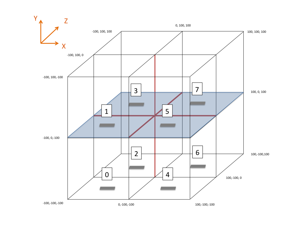
A typical space in 3-D, using 2 x 2 x 2 process, looks like this:
In this case we have defined a space that runs from -100 to 100 in the x, y, and z dimensions. This space is divided among 8 processes, so that each process manages a 100 x 100 x 100 portion. The numbers inside these portions indicate the processor number assigned to that portion. Importantly, the assignment of process numbers is arbitrary; it cannot be assumed that this will be the same from run to run. (It will very likely be consistent, but this is ultimately driven by the MPI implementation, and therefore cannot be assumed.)
Recall that in the 2-D case, a given process would have 8 neighbors. See for a refresher. For the N-Dimensional case, the 8 neighbors are increased; the number of neighbors is always (3^N) - 1. The derivation of this is that in each dimension there is, essentially, a -1 (left), 0 (alongside) and 1 (right) case, and the total number of cases is the product of this in all dimensions, minus the central cell. For the 2-D case this is a simple 3 x 3 'tic-tac-toe' board with the center cell removed. In 3 dimensions it becomes like a Rubik's cube, but with the (usually unseen) center cube removed.
The examples we have used in the 2-D case have had only four processes but toroidal boundaries; hence the 8 neighbors of a given process must be the other three, and (because 8 is more than three!), some of the processes have to be neighbors twice. In the 2-D case, Process 1's von Neumann neighbors (N-S and E-W) were Process 3 and Process 0, which were each used twice, and Process 2, which was on all four corners. The 3-D case is more complicated, but analogous: in the diagram above, Process 1's 'full-face' neighbors would be Process 5 (above it and below it in the X dimension), Process 0 (above it and below it in the Y dimension), and Process 3 (above it and below it in the Z dimension). It would additionally be neighbors along four joints each with Processes 7, 4, and 2. Finally, at each of its 8 corners it would see Process 6. The total number of 'neighbors' is (2 + 2 + 2 + 4 + 4 + 4 + 8 = 26 = 3 ^ 3 - 1).
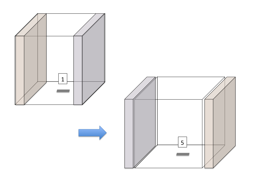
The division of space into 'buffer zones' in N-Dimensions exactly parallels the way that it is divided in 2-Dimensions: on the inside of the space's local boundaries there is a zone that is copied to all neighboring processes. The difference is that in N-Dimensional space these zones are, properly, N-Dimensional volumes. In higher dimensions this becomes even more difficult to visualize, but the basic principle remains the same. If the processors are organized as in the figure above, Process 1 must send full faces to Process 5, Process 0, and Process 3. This is illustrated for Process 5 as:
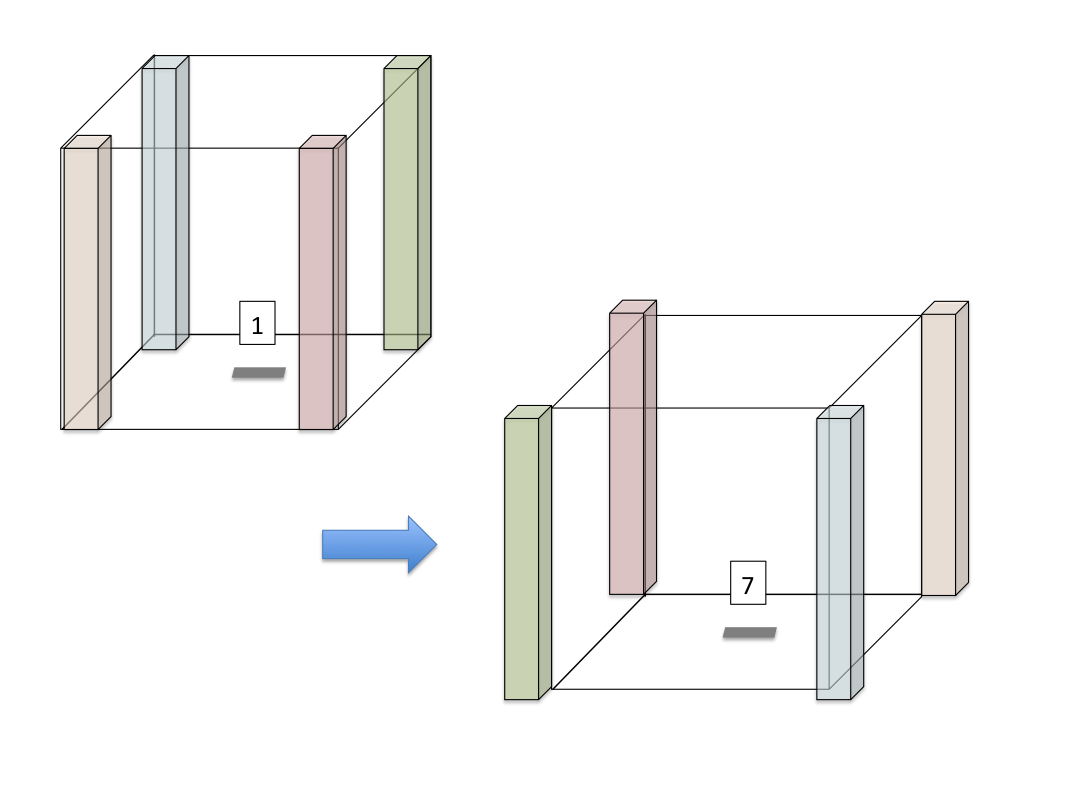
Process 1 must also send edges to Process 7, Process 2, and Process 4. This is depicted for Process 7 as:
Finally, Process 1 must send its corners to Process 6:
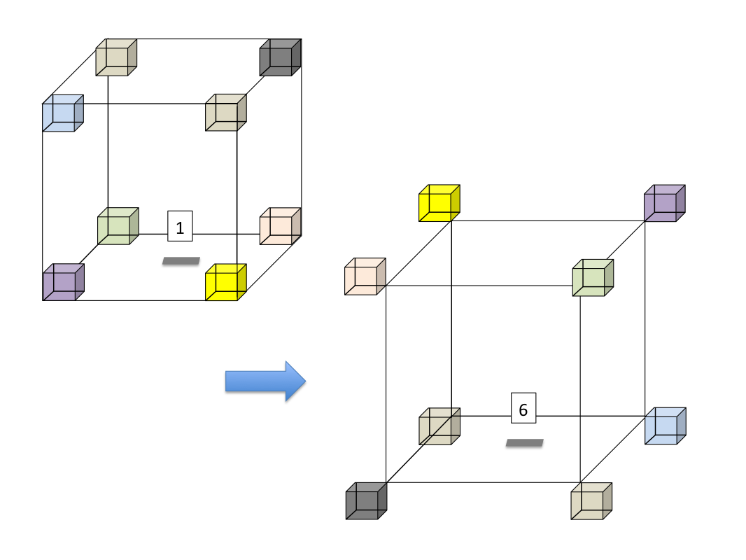
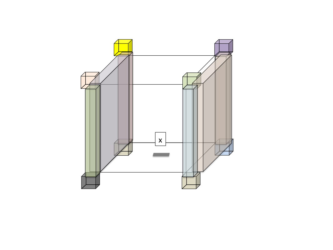
A cell that is receiving this information assembles it into a complete picture of the volume of space around it. In this image, the cell for Process 'x' has received two faces, four edges, and all eight corners; the rest of the volume is omitted for clarity, but would form a complete 'shell' around the central cell:
All of the rules about local vs. non-local agents in 'buffer zones' presented with respect to 2-D spaces remain identical in N-Dimensions.